Tutorial on Numerical Methods #2 for Fiber Optics Gain Simulator by Using Python #Tutorial-8

What Will I Learn?

This tutorial continues the topics on scientific calculations such as simplification, expansion, differentiation, integration and solving equations by using sympy packages. This package is about symbolic calculations. Before continuing the previous tutorial which is about Fiber Optics Gain Simulator, we need to learn these calculations also.

• You will learn how to use .Symbol and .symbols method to create symbols
• You will learn how to create functions by using symbols.
• You will learn how to use .subs method to solve functions by real values.
• You will learn how to use .pprint method to see the functions into real form.
• You will learn how to use .simplify, .factor and .expand methods to simplify, factor and expand the functions respectively.
• You will learn how to use .diff method to take differentiation of the functions.
• You will learn how to use .integral method to take integral for the functions.

Requirements

• Windows 8 or higher.
• Python 3.6.4.
• PyCharm Community Edition 2017.3.4 x64.
• Importing sympy

Difficulty

This tutorial has an indermadiate level.

Tutorial Contents

In this tutorial, we will learn how to calculate the functions by using symbols such as implification, expansion, differentiation, integration and solving equations. To solve equations, using symbols are really easy to do that. If you have a equation which can includes integral, differentiations also, you can solve it easily by using symbols.

First of all, we need to import the sympy package such that:

import sympy as sym

For sympy package we will assign a name such as sym instead of writing sympy package.

Now, we can define our symbols by using .Symbol method for one symbol and .symbols method for multiple symbols such as:

a = sym.Symbol('a')
b,c,d = sym.symbols('b,c,d')

Then, we define our functions in two ways, first one is .Function method and the other one is just wirting the equations such that:

func1=sym.Function('f')
func2=x**4+y**3+z**2+t**1

If you want to see the functions you can see it by using print method which will show general equation or for mathematical method you can use .pprint method such that:

a**4 + b**3 + c**2 + d ---- print method

  4      3      2    
a  + b  + c  + d ---- pprint method

Now, we are ready to write our functions and solve it. We will use func2 to solve first example. For example for a=1, b=2, c=3, d=4 then calculate the func2.
You can use .subs method such that, nameofFunction.subs({variable:worth, ....}) and also you can change your variable name as well such that:

func2=a**4+b**3+c**2+d**1
sym.pprint(func2.subs({a:1, b:2, c:3, d:4}))
sym.pprint(func2.subs({a:x, b:y, c:z, d:t}))

The result:

22
          4     3     2
t + x  + y  + z 

Let's start with simplification of a function which is (x³+3x²+3x¹+1)//(x+1) by using .simplify method. Then we will factor of this solution by using .factor method and then we will expand it again by using .expand method.

func3=(x**3+3*x**2+3*x**1+1)/(x+1) # our new function
sym.pprint(sym.simplify(func3)) # simplification
func4=sym.simplify(func3) # simplified function
sym.pprint(sym.factor(sym.factor(func3))) # factoring
func5=(sym.factor(sym.factor(func3))) # factored function
sym.pprint(sym.expand(func5)) # expansion

The result:

  2          
x  + 2⋅x + 1 --- simplification
            2
(x + 1)  ---- factoring
  2          
x  + 2⋅x + 1 ---- expansion

Also you can solve differentiation by using .diff method such that:

func6=(sym.sin(x)*(sym.cos(x))**2)
sym.pprint(func6)
difFunc=sym.diff(func6,x)
sym.pprint(difFunc)

       2   
sin(x)⋅cos (x)
              2                               3   
- 2⋅sin (x)⋅cos(x) + cos (x)

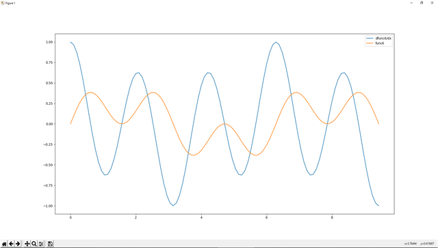
As you see .diff method is used like this, **diff(function,dx). Let's see its numerical calculation on graph.

func6=(sym.sin(x)*(sym.cos(x))**2)
sym.pprint(func6)
difFunc=sym.diff(func6,x)
sym.pprint(difFunc)
a=importing.linspace(0,3,100)
resultfunc6=[]
resultDiff=[]
for i in range(100):
    resultfunc6.append(func6.subs(x,a[i]*sym.pi))
    resultDiff.append(difFunc.subs(x,a[i]*sym.pi))
plotting.plot(a*sym.pi,resultDiff,label='dfunc6/dx')
plotting.plot(a*sym.pi,resultfunc6,label='func6')
plotting.legend()
plotting.show()

The result:

As you see that you can assign real number to your variables by using .subs method.

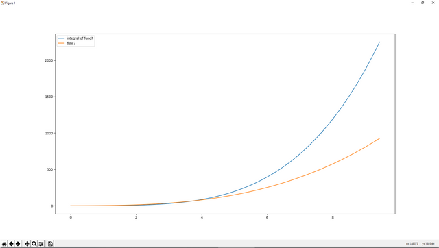
Let's do integration for our new function which is func7 by using .integrate method such as:

func7=x**3+x**2
sym.pprint(func7)
integFunc=sym.integrate(func7,x)
sym.pprint(integFunc)
resultIntegral=[]
resultfunc7=[]
for i in range(100):
    resultIntegral.append(integFunc.subs(x,a[i]*sym.pi))
    resultfunc7.append(func7.subs(x,a[i]*sym.pi))
plotting.plot(a*sym.pi,resultIntegral,label='integral of func7')
plotting.plot(a*sym.pi,resultfunc7,label='func7')
plotting.legend()
plotting.show()

The result:

  3     2
x  + x 
      2      
3⋅x  + 2

Let's move on solution of equations. First of all, we will try to solve a simple equation by using .Eq method. Then, we will evaluate the solution to get float solution by using .evalf method such that:

Eqn1=sym.Eq(x**2+2*x+1,x+2)
sym.pprint(Eqn1)
solution1=sym.solve(Eqn1,x)
sym.pprint(solution1)
# to see float solution
print(solution1[0].evalf())
print(solution1[1].evalf())
# or to see float solution
for i in range(len(solution1)):
   print(solution1[i].evalf())

The result:

# equation
  2                  
x  + 2⋅x + 1 = x + 2

# solution
⎡  1   √5    √5  1⎤
⎢- ─+─, - ─ - ─⎥
⎣  2     2     2     2⎦

# float solution 
0.618033988749895
-1.61803398874989
# float solution by using for loop
0.618033988749895
-1.61803398874989

Let's make a little bit hard equation which includes 3 unknowns.
Eqn1=x+y+z=0
Eqn2=2x+10y+z=100
Eqn3=4x+5z=-40
Such that:

Eqn2=sym.Eq(x+y+z,0)
Eqn3=sym.Eq(2*x+10*y+z,100)
Eqn4=sym.Eq(4*x+5*z,-40)
sym.pprint(sym.solve([Eqn2,Eqn3,Eqn4],[x,y,z]))
solution2=(sym.solve([Eqn2,Eqn3,Eqn4],[x,y,z]))

The result:

x + y + z = 0 ---- Equation-1
2⋅x + 10⋅y + z = 100 ---- Equation-2
4⋅x + 5⋅z = -40 ---- Equation-3
{x: -35, y: 15, z: 20} ---- Solution

The usage of .solve method for multiple variables is like this. You need to write the equations inside your method and you need to write the variables which must be solved such that, .solve([Equations],[Variables]).

Also you can write these equations into matrix form. For example for
Eqn1=x+y+z=0
Eqn2=2x+10y+z=100
Eqn3=4x+5z=-40
You can for a matrix;

•                                                                   [1  1  1]
  

•                                           MatrixA=    [2 10 1]
  

•                                                                   [4   0  5]
  

And the results are;

•                                                               [0]
  

•                                         Result=  [100]
  

•                                                             [-40]
  

matrixA=sym.Matrix([[1,1,1],[2,10,1],[4,0,5]])
resultA=sym.Matrix([[0],[100],[-40]])
sym.pprint(matrixA)
sym.pprint(resultA)

The matrix are:

# matrixA
⎡1    1   1⎤
⎢                ⎥
⎢2  10  1⎥
⎢                ⎥
⎣4    0   5⎦
# resultA
⎡    0  ⎤
⎢         ⎥
⎢100⎥
⎢         ⎥
⎣ -40⎦

As you see, to form matrix you can use .Matrix method and for each row you need write into brackets. For each column you need to seperate them by , into the row.

To solve the matrix equations you need to use .LUsolve method such that:

sym.pprint(matrixA.LUsolve(resultA))


⎡-35⎤
⎢        ⎥
⎢15  ⎥
⎢        ⎥
⎣20  ⎦

As you see you can solve equations by matrix method also.

In this tutorial, we learnt scientific calculations such as simplification, expansion, differentiation, integration and solving equations by using sympy packages which is related to symbolic calculations.

Curriculum

Here is the list of related tutorials we have already shared on @utopian-io community.

• Tutorial on Numerical Methods for Fiber Optics Gain Simulator by Using Python #Tutorial-7
• Tutorial on Fiber Optics Gain Simulator by Using Python #Tutorial-6
• Tutorial on Plotting by Using matplotlib Package and Giving an Example of FFT Analysis in Python #Tutorial-5
• Tutorial on GUI (continues) and Example of Web Crawler by combining PyQt5 and BeautifulSoup package in Python #Tutorial-4
• Tutorial on GUI and Example of Simple Addition Calculator by using PyQt5 package in Python #Tutorial-3
• Creating Package and Subpackage in Python #Tutorial-2
• Example of Steemit Analysis by Using Python #Tutorial-1

---

Posted on Utopian.io - Rewarding Open Source Contributors

---