Data Analysis with Google Sheets: (Advanced Excel Formulas, and Pivot Tables )

lhorgic (76)in #spreadsheet-s20w2 • 2 months ago

Hello guys! Good to have y'all here once again, it's my pleasure to participate once again in this class. I must confess, I loved what we discuss last week being the introductory part of the lecture. I had already purposed in my heart that I am going to follow this course to the end because for me it something I need career wise. Anyways let me cut the story short as I get into the business of the day.

^{Explain what you understand by Advanced Excel Formulas, and show us where advanced formulas such as the lookup function, and logical function are found in Excel with clear screenshots.}

Advance Excel Formulas are those in built formulas we have on excel used to carry out special functions on excel. It is called advanced because it more sophisticated than the usual fomular we are familiar with just like the SUM function, AVERAGE function and and a host of others.

Advance Excel Formulas help us in filtering data, duplicating data, carrying out retrieving functions amongst other special functions. These formular seem to be less maximized on spreadsheet and this could be as a result of the little knowledge people have about it. Am really glad we would be exploring these formulas in this lesson.

I think it would also be expedient I mention some of these advance formulas even before I go ahead to show us where they can be found in our spreadsheet. Although I will be mentioning just a few which we can find below.

• VLOOKUP
• HLOOKUP
• GETPIVOTDATA
• IF LOGICAL FUNCTION
• IF ERROR LOGICAL FUNCTION etc

Below is how to locate these advance formulas on our spreadsheet.

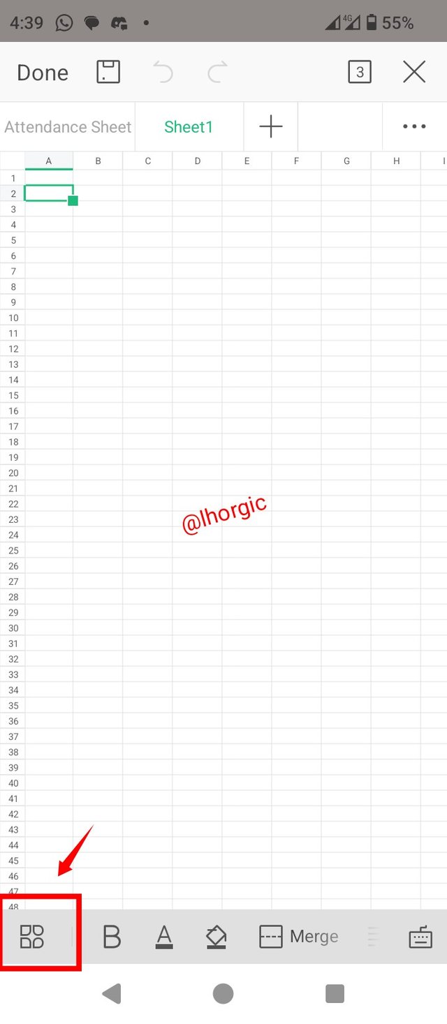
• Step 1: I Launched my spreadsheet and clicked the menu icon.

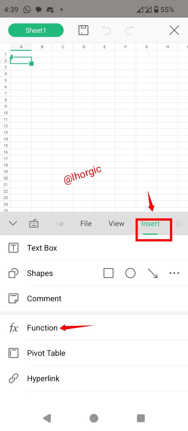
• Step 2: I located my insert icon and clicked on it.

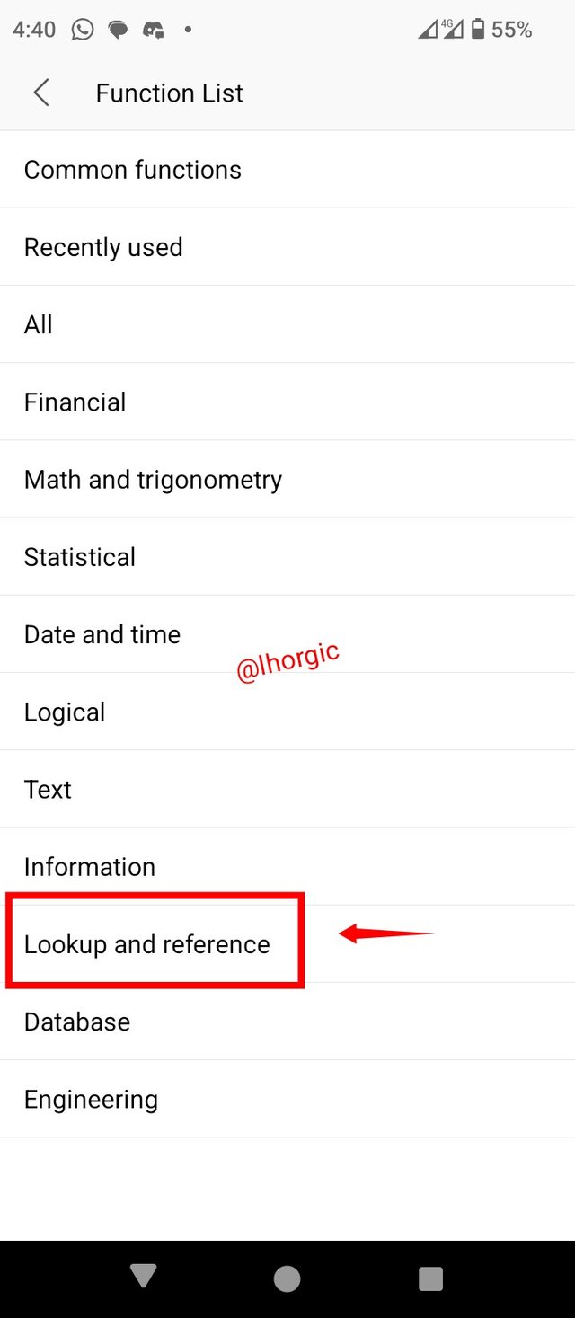
• Step 3: I located the Lookup and reference section and clicked it.

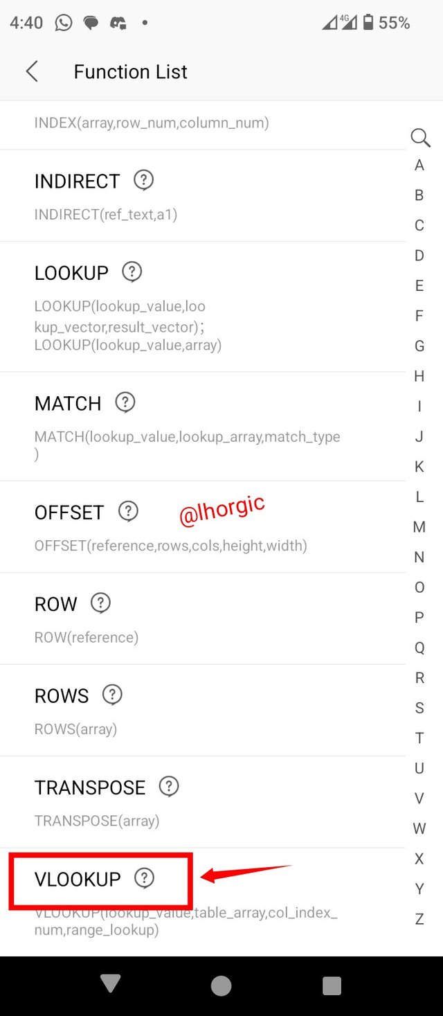
• Step 4: I was brought to this I terface where I scrolled down to locate my VLOOKUP.

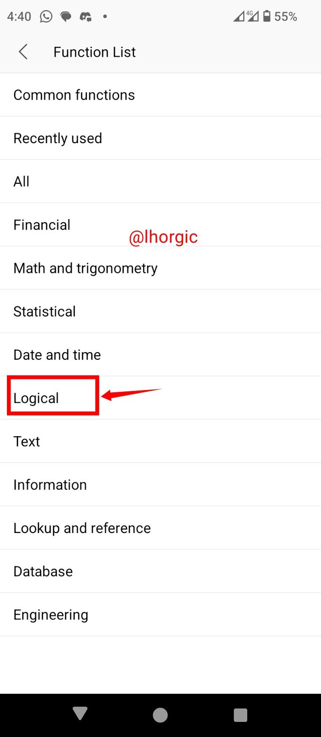
• Step 6: I came back to the different sections we have and then located the Logical section.

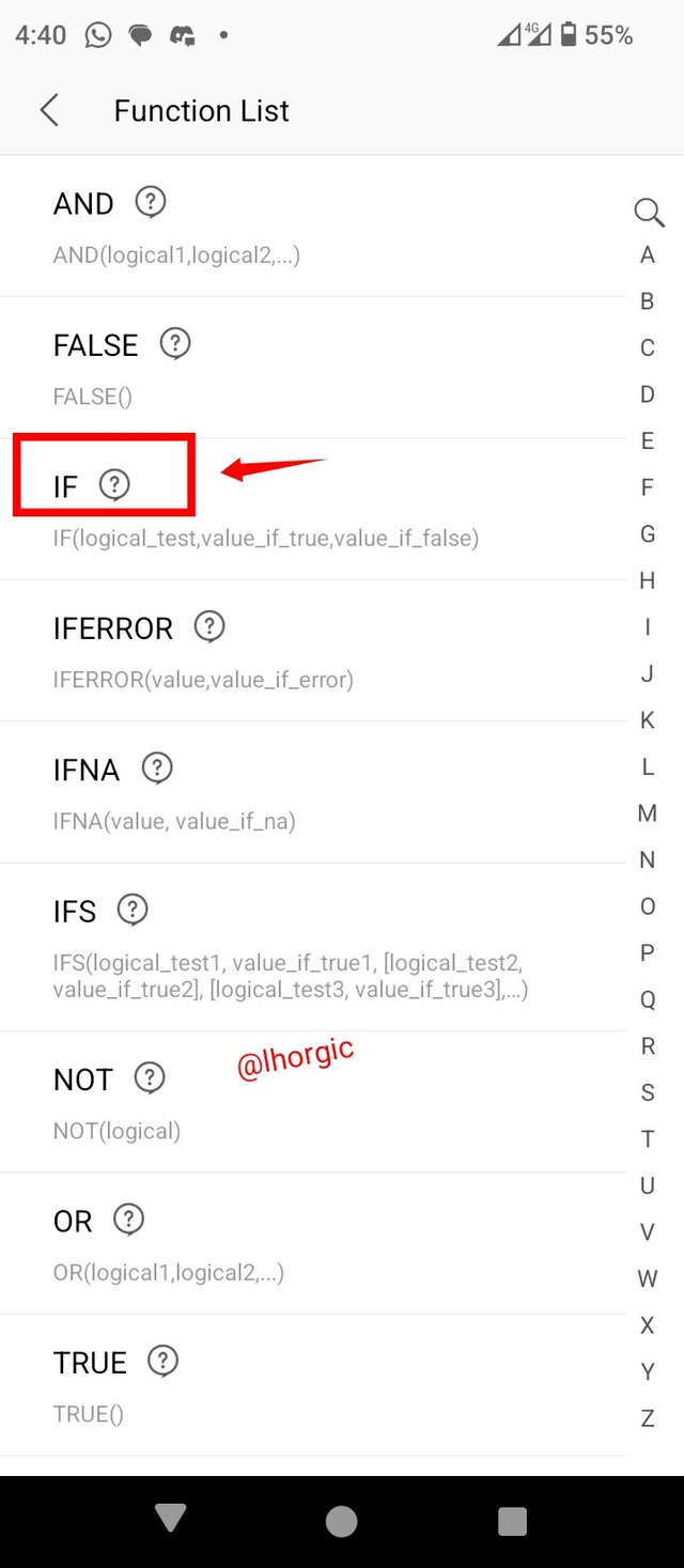
• Step 7: I clicked it and then scroll it locate the if function just as seen.

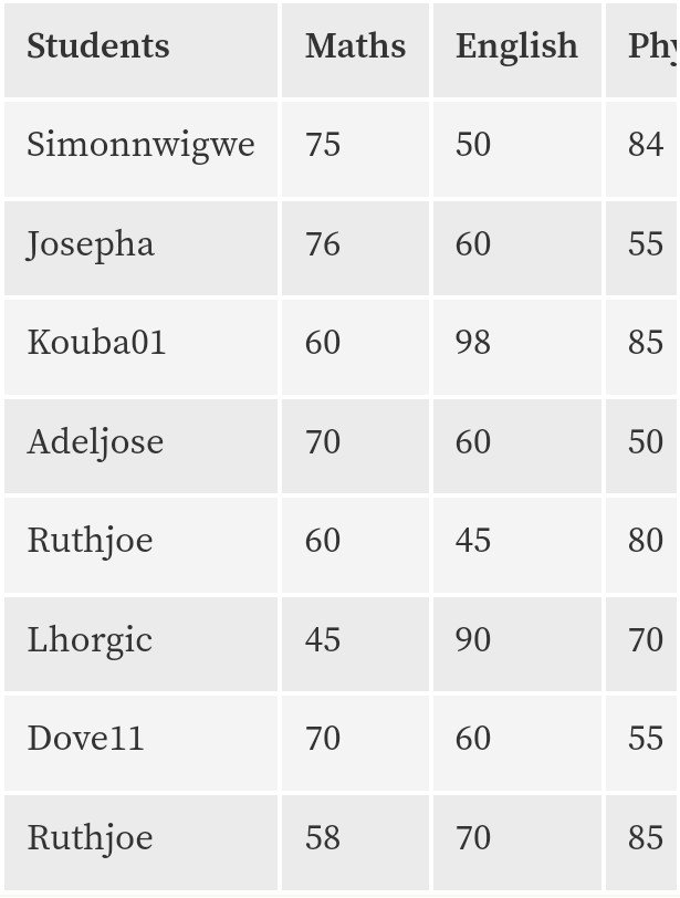
^{Write the "IF" Function formula to calculate the total, average score, and grade of students given in the table below.}

In the section we want to explore the use of the "If" function coupled with the total and average function. Having learnt so much from my teacher, I would love to practically carry out what I've learnt using the table given to us in the homework task...this can be found below.

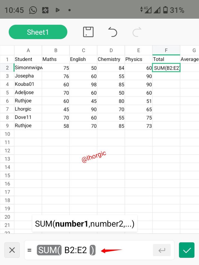
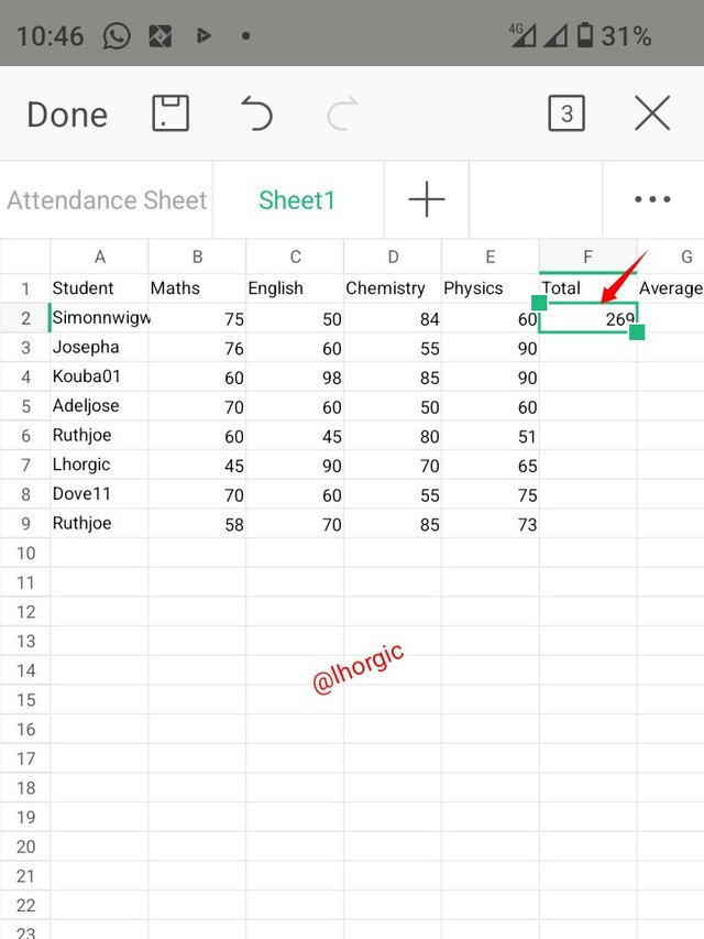
I would love to start with the "Total". From the last class we were taught the use of SUM which can help us get our total as total simply means the summation of the values in the cell. This time it the sum of cell B2, C2, D2, E2 which can be written like as = SUM (B2:E2) in our formular bar.

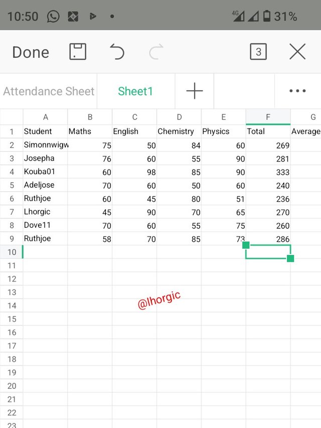
That was was what I used to derive the first and then repeated the process for the next using = SUM (B3:E3), = SUM (B4:E4), = SUM (B5:E5), = SUM (B6:E6), = SUM (B7:E7), = SUM (B8:E8), = SUM (B9:E9). The corresponding outcome is also as seen in my screenshot below.

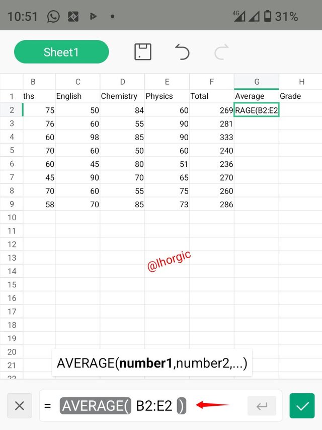
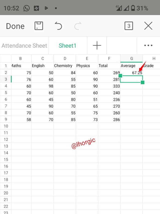
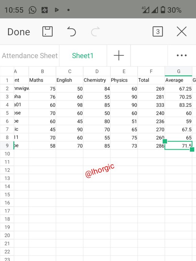
I then moved to the average function. We also learnt about this function last week and it has also stuck in my memory since then, am even liking the fact that we have to build on the previous lesson. The formula given is = AVERAGE(B2:E2). This give us the average of the sum total of the cell. The same was used for the other i.e = AVERAGE(B3:E3) = AVERAGE(B4:E4) ,
= AVERAGE(B5:E5) etc. The process is as seen below.

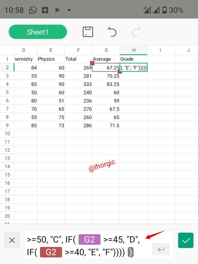
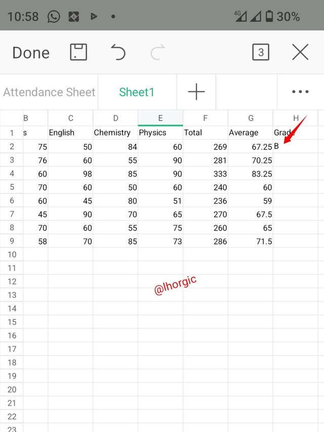
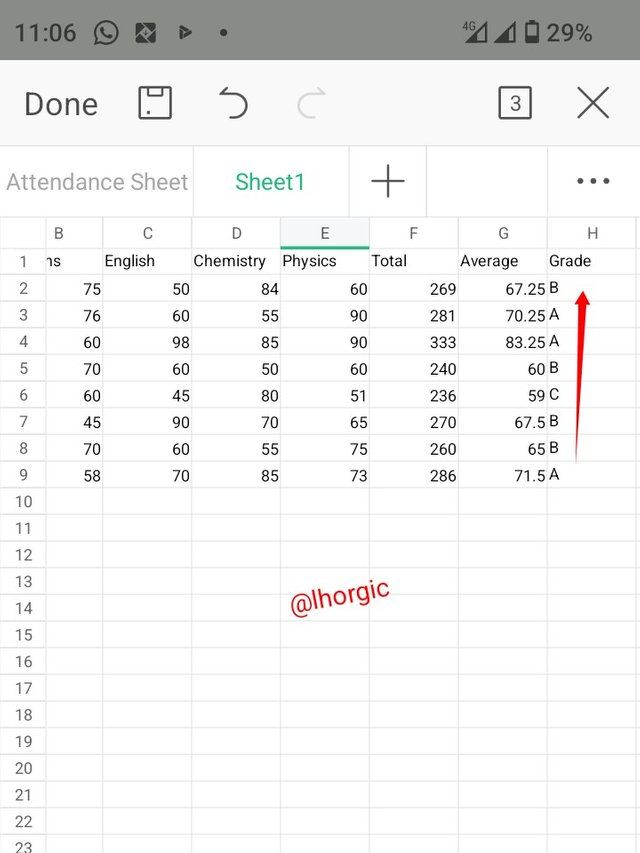
I then proceeded to the IF function which is a conditional statement that should give us our desired result when conditions are met or not as the case may be. It was applied just as we were taught by our teacher and of course I demonstrated it just as seen in my image below.
The formula used is this.=IF(G2>=70, "A", IF(G2>=60, "B", IF(G2>=50, "C", IF(G2>=45, "D", IF(G2>=40, "E", "F"))))). I also used the same formular to get the rest of the student. Here are the fomulars
=IF(G3>=70, "A", IF(G3>=60, "B", IF(G3>=50, "C", IF(G3>=45, "D", IF(G3>=40, "E", "F"))))), =IF(G4>=70, "A", IF(G4>=60, "B", IF(G4>=50, "C", IF(G4>=45, "D", IF(G4>=40, "E", "F"))))) e.t.c.

Here is the practical steps of applying the if function.

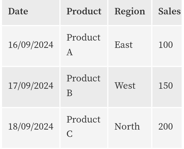
^{Based on the given data below: Create a pivot table that shows (see) total sales by product, by dragging the product to the Rows areas, Region to the Column area, and Sales to the Values area. Please we want to see the steps you take in adding your pivot table.}

In this section I want to practically put into practice what our teacher taught us about pivot table. I had to carefully try this out because it seems to be the tasking part of this homework task. However after thoroughly going through what I learn I came up with the following using the table below.

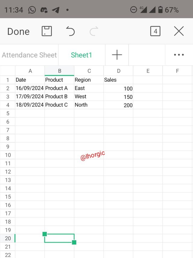
• Step 1: I input all the data just as given in the table above.

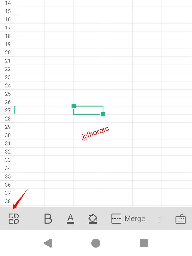
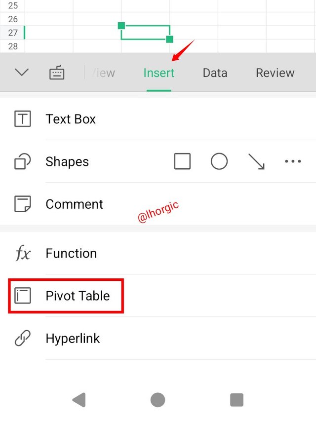
• Step 2: I went in search of my pivot table by going to the menu bar, located my insert icon and then scrolled down to get my pivot table.

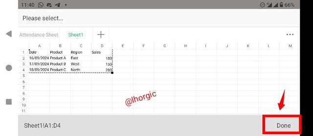
• Step 3: I highlight the field where I have all my items and then click done.

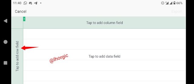
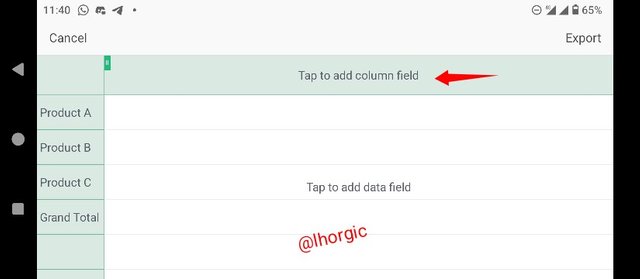
• Step 4: I click on the column section so that I can fill in the field.

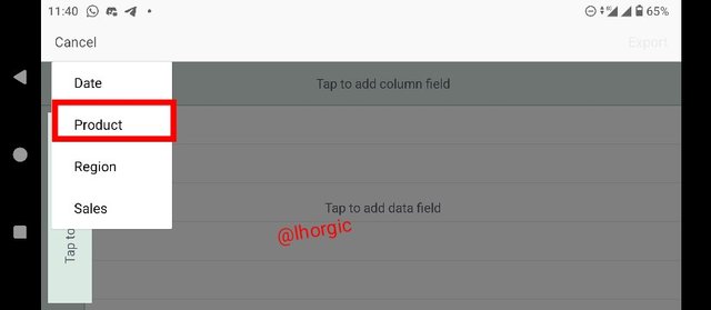
• Step 5: a list of action popped up after clicking the column section...from which I chose "Product"

• Step 6: I clicked on the Row section as well so I can fill in the item that should be there.

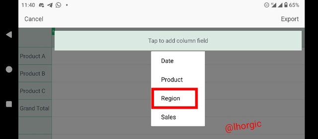
• Step 7: a list of action popped up after clicking the Row section...from which I chose "Region" just as seen

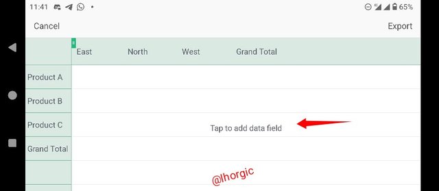
• Step 8: I then click on the "add to data field" to fill up the content.

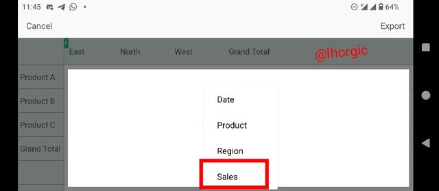
• Step 9: a list of action popped up after clicking the "add to field" section...from which I chose "Sales" just as seen

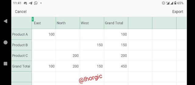
• Step 10: This gave us the final result of everything we have put together.

This brings us to the end of the demonstration on how to use the pivot table for our analysis. I hope I have been able to show in details how I was able to achieve all of these. Let me specially appreciate our teacher for this lecture, it's indeed loaded and educative. I have purposed in my heart to follow the lecture all the way. I really do hope I am able to achieve this.

Just before I drop my pen, I would like to invite @okere-blessing @drhira @waqarahmadshah. I hope they find these lecture interested.

Regards
@lhorgic❤️

#burnsteem25 #learnwithsteem #steemexclusive #club5050 #nigeria