SEC | S20W2 |Data Analysis with Google Sheets: (Advanced Excel Formulas, and Pivot Tables )

_{Edited By Canva}

Hello steemians,

For this contest, I will demonstrate my skills in data analysis using Google Sheets, advanced Excel formulas, and pivot tables, leveraging the French version of Excel. Throughout my work, I utilize a variety of powerful Excel functions to manage and analyze data effectively. Whether it’s performing complex calculations with advanced formulas or summarizing large datasets with pivot tables, I will showcase how these tools help streamline the analysis process.

By participating in this contest, I aim to highlight the adaptability of Excel for data analysis, whether in English or French, and provide insights into how these advanced tools help transform raw data into meaningful reports.

Explain what you understand by Advanced Excel Formulas And Show us where advanced formulas such as the lookup function, and logical function are found in Excel with clear screenshots.

For me, advanced Excel formulas are powerful tools that allow me to manipulate and analyze data efficiently. They go beyond basic arithmetic and enable me to perform complex calculations, automate tasks, and extract valuable insights from large datasets. One of the key aspects of advanced formulas is the ability to combine multiple functions to solve complex problems.

Advanced Excel Formulas

In this image, the Formulas tab of Excel is highlighted, showing different categories of advanced Excel functions. The main categories include:

• Financial: Used for financial calculations like loan payments, interest rates, and depreciation.
• Logical: Functions that allow logical comparisons and decision-making (e.g., IF, AND, OR).
• Text: Functions that manipulate text strings (e.g., CONCATENATE, LEFT, RIGHT).
• Date & Time: Functions for handling date and time operations (e.g., TODAY, NOW).
• Lookup & Reference: Functions to search for data within a table or range (e.g., VLOOKUP, HLOOKUP, INDEX, MATCH).
• Math & Trigonometry: Functions to perform mathematical calculations (e.g., SUM, PRODUCT, SIN, COS).
  These categories offer quick access to different types of formulas depending on the task at hand.

For instance, I often use the lookup functions like VLOOKUP, HLOOKUP, INDEX, and MATCH to search for specific data within a range and return corresponding values. These formulas are beneficial when I need to cross-reference large tables or perform database-like operations. The lookup functions are under the Formulas tab in Excel, specifically in the Lookup & Reference category.

Lookup Functions

The image shows the Lookup & Reference section, which contains several important lookup functions, such as:

• VLOOKUP: Used to search for a value vertically in a table.
• HLOOKUP: Similar to VLOOKUP, but searches horizontally.
• INDEX: Returns the value of an element in a table or array, based on the row and column numbers.
• MATCH: Searches for a specified item in a range and returns the relative position.
  These functions are essential for retrieving data from large datasets based on specific criteria.

Another important category of advanced formulas I rely on includes logical functions such as IF, AND, OR, and NOT. These allow me to create conditional logic within my worksheets. For example, I can use the IF function to instruct Excel to perform different calculations based on specific conditions. These logical functions can be found under the Formulas tab in the Logical category.

Logical Functions

This image highlights the Logical Functions dropdown under the Formulas tab. Some of the functions visible include:

• IF: A logical function that returns one value if a condition is true and another value if it's false.
• AND: Returns TRUE if all arguments are true.
• OR: Returns TRUE if at least one argument is true.
• NOT: Inverts the logical value.
  These logical functions are essential for decision-making in Excel, allowing the user to perform conditional operations and validate data.

Write the IF Function formula to calculate the total, average score, and grade of students given in the table below.

1. Sum of Scores

This table focuses on calculating the total score for each student, which is the sum of the scores in Maths, English, Physics, and Chemistry. The formula used for this is =SOMME(B2:E2) in column F.

• Example:
  • Simonwigwe has the following scores: 75 in Maths, 50 in English, 84 in Physics, and 60 in Chemistry, giving a total of 2175.

2. (Average Calculation)

This table displays students' grades in four subjects: Maths, English, Physics, and Chemistry. For each student, the total score (sum of the scores from the four subjects) is calculated in column F, and the average score is calculated in column G. The formula used for the average in cell G2 is =MOYENNE(B2:E2), which calculates the average of the grades from columns B (Maths) to E (Chemistry). The average is then used to assign a grade in column H. The grades range from A to F, based on the student's average score.

• Example:
  • Simonwigwe scored 75 in Maths, 50 in English, 84 in Physics, and 60 in Chemistry. The total score is 2175, and the average is 67.25, giving him a grade of B.

3. Nested IF Function with Conditions

This table showcases how the IF function is used to assign grades based on average scores. The formula in cell H2 is a nested IF function:

=SI(G2>=70,"A",SI(G2>=60,"B",SI(G2>=50,"C",SI(G2>=45,"D",SI(G2>=40,"E","F")))))

This formula checks the student's average in column G and assigns a grade based on specific thresholds. For example:

• If the average is 70 or above, the student gets an A.

• If the average is between 60 and 69, the student gets a B, and so on.

• Example:

  • Ruthjoe, with an average of 59, is assigned a grade of C.

4. Final Graded Table

This table includes the same student list with their scores in four subjects, and it provides additional columns for the total score, average, and grade. The grades are assigned based on specific conditions tied to the average score:

• A if the average is 70 or higher.
• B if the average is between 60 and 69.99.
• C if the average is between 50 and 59.99.
• D, E, and F for lower ranges.

The formula for the total score is =SOMME(B2:E2), and the formula for the average is =MOYENNE(B2:E2).

• Example:
  • Josepha has a total of 1906 points with an average of 70.25, receiving a grade of A.

Briefly discuss four IF function Operators that you have learned and tell us their functions and when we are to use them.

I will discuss the four main operators: logical, comparison, mathematical, and text operators, using specific scenarios.

1. Logical Operators

Logical operators are used to combine multiple conditions into an IF formula. I often use them when I need to evaluate complex scenarios that require multiple criteria to determine the outcome.

Example: In a student tracking table, I need to check if each student has achieved the minimum grades required to pass. The criteria are: Math ≥ 70, Physics ≥ 80, and Chemistry ≥ 65.

Formula: =IF(AND(B2>=70;C2>=80;D2>=65);"Pass";"Not Pass")

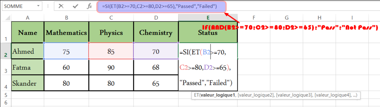
Result: If all conditions are met, the student is marked as "Pass", otherwise "Not Pass".

I use logical operators when I need to check multiple conditions that must all be true for a specific outcome, like ensuring students meet all score requirements to pass.

2. Comparison Operators

Comparison operators are used to compare two values. I often use them to evaluate simple conditions.

Example: I want to check if a user has voted exactly 100 times in a competition to mark them as "Qualified".

Formula: =IF(A2=100;"Qualified";"Not Qualified")

Result: If the number of votes is equal to 100, the user is marked "Qualified".

I use comparison operators when I want to evaluate a straightforward condition like checking for an exact value or range in a data set.

3. Mathematical Operators

Mathematical operators allow me to perform simple calculations like addition, subtraction, etc., directly in an IF function.

Example: In a table tracking the publication of articles, I need to check if a Steemian has written at least 20 articles in four weeks to be considered "ACTIVE".

Formula: =IF(B2+C2+D2+E2>=20;"ACTIVE";"NOT ACTIVE")

Result: If the total of articles over four weeks is greater than or equal to 20, the Steemian is marked "ACTIVE".

I use mathematical operators when I need to total values or perform other simple calculations to determine a condition, like the total number of articles written over a certain period.

4. OR Operator

The OR operator allows me to test multiple conditions and return a result if at least one of the conditions is true. It's particularly useful when I need to validate scenarios where several options are possible.

Example: I need to check if a student has passed based on a more flexible rule. The student must score at least 70 in Mathematics or at least 80 in Physics to be considered "Passed."

Formula: =IF(OR(B2>=70, C2>=80), "Passed", "Failed")

Result: If the student meets at least one of the two conditions (Math ≥ 70 or Physics ≥ 80), they are marked "Passed." Otherwise, they are marked "Failed."

I use this operator when I want to validate multiple possibilities, such as when I want to allow some flexibility in evaluation criteria. It’s useful in scenarios where one or the other condition can be enough to get a positive result.

This operator simplifies my calculations when several outcomes can be considered acceptable, unlike the AND operator, which requires all conditions to be true.

Based on the given data below: Create a pivot table that shows (see) total sales by product, by dragging the product to the Rows areas, Region to the Column area, and Sales to the Values area. Please we want to see the steps you take in adding your pivot table.

Based on the pivot table creation process illustrated in the screenshots, here's a detailed step-by-step description of how I created the pivot table, using the pronoun "I":

Step 1: Prepare the Data

I start by having my dataset in place. It consists of four columns: Date, Product, Region, and Sales, showing the sales data for different products across various regions. The table includes entries for:

• Product A (East, 100 units)
• Product B (West, 150 units)
• Product C (North, 200 units)

Step 2: Select the Data for the Pivot Table

I select the entire table by dragging my cursor across the data range from A1 to D4. This ensures that all the relevant fields (Date, Product, Region, and Sales) are selected for analysis in the pivot table.

Step 3: Insert a Pivot Table

I navigate to the "Insertion" tab in Excel, where I choose "Tableaux croisés dynamiques" (Pivot Table) from the available options. This opens a dialog box, asking me to confirm the data range and the location for the new pivot table. I opt to create the pivot table in the existing sheet, placing it starting at cell B8.

Step 4: Configure the Pivot Table Fields

In the pivot table configuration window on the right, I begin adding fields to the pivot table by dragging and dropping them:

• Product goes into the Rows area, so each product (A, B, C) is listed in the pivot table rows.
• Region goes into the Columns area, displaying each region (East, West, North) across the top of the table.
• Sales is added to the Values area, summing the total sales for each product and region.

Step 5: View the Pivot Table

Once I’ve arranged the fields correctly, the pivot table starts to take shape. It shows a breakdown of sales for each product across the three regions. For example:

• Product A sold 100 units in the East.
• Product B sold 150 units in the West.
• Product C sold 200 units in the North.

Step 6: Final Pivot Table View

In the final version of the pivot table, I can see the total sales for each product, as well as the Grand Total for all regions combined, which amounts to 450 units. The rows and columns are neatly organized, making it easy to analyze the sales data by product and region.

This pivot table provides a clear overview of how each product is performing in different regions, helping me quickly analyze and summarize the sales data.

---

Thank you very much for reading, it's time to invite my friends @lil.albab, @miftahulrizky, @heriadi to participate in this contest.

Best Regards,
@kouba01