Machine Learning Series (Support Vector Machines)
Introduction
In this series of posts, I'll introduce the theory behind Support Vector Machines, a class of machine learning algorithms used for classification purposes.
1.0 Support Vector Machines
Support Vector Machines (SVMs) is a machine learning algorithm used for classification tasks. Its primary goal is to find an optimal separating hyperplane that separates the data into its classes. This optimal separating hyperplane is the result of the maximization of the margin of the training data.
1.1 Separating Hyperplane
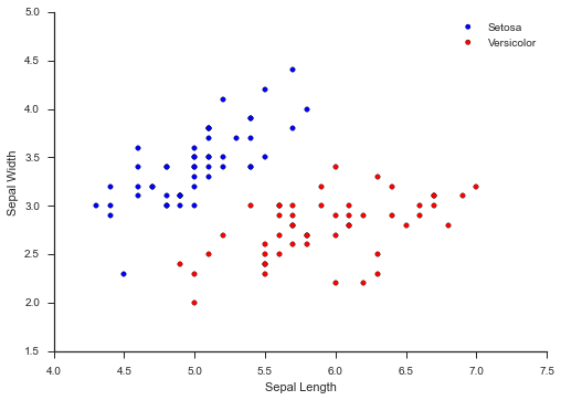
Let's take a look at the scatterplot of the iris dataset that could easily be used by a SVM:
Just by looking at it, it's fairly obvious how the two classes can be easily separated. The line which separates the two classes is called the separating hyperplane.
In this example, the hyperplane is just two-dimensional, but SVMs can work in any number of dimensions, which is why we refer to it as hyperplane.
1.1.1 Optimal Separating Hyperplane
Going off the scatter plot above, there are a number of separating hyperplanes. The job of the SVM is find the optimal one.
To accomplish this, we choose the separating hyperplane that maximizes the distance from the datapoints in each category. This is so we have a hyperplane that generalizes well.
1.2 Margins
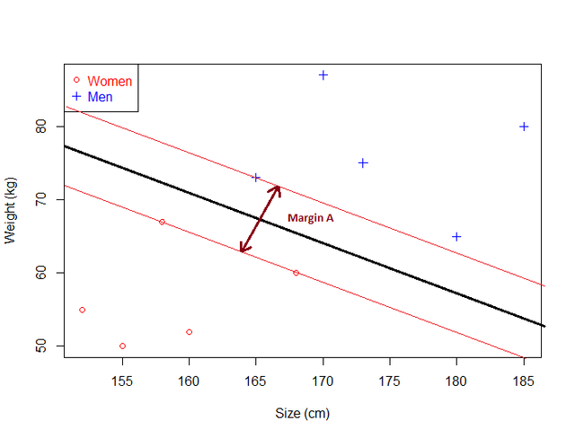
Given a hyperplane, we can compute the distance between the hyperplane and the closest data point. With this value, we can double the value to get the margin. Inside the margin, there are no datapoints.
The larger the margin, the greater the distance between the hyperplane and datapoint, which means we need to maximize the margin.
1.3 Equation
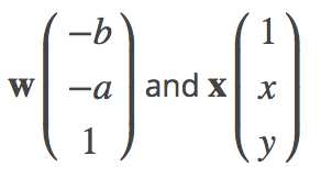
Recall the equation of a hyperplane: wTx = 0. Here, w and x are vectors. If we combine this equation with y = ax + b, we get:
This is because we can rewrite y - ax - b = 0. This then becomes:
wTx = -b Χ (1) + (-a) Χ x + 1 Χ y
This is just another way of writing: wTx = y - ax - b. We use this equation instead of the traditional y = ax + b because it's easier to use when we have more than 2 dimensions.
1.3.1 Example
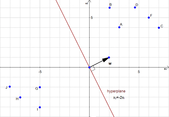
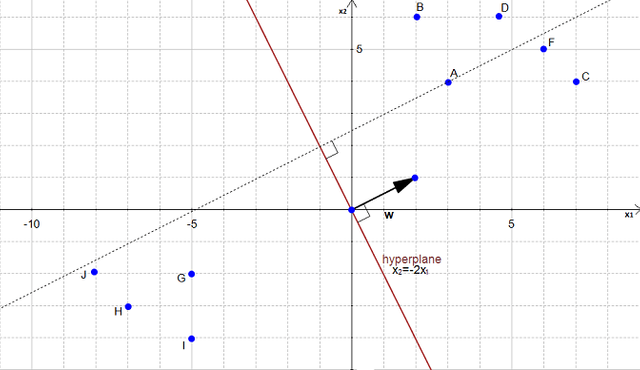
Let's take a look at an example scatter plot with the hyperlane graphed:
Here, the hyperplane is x2 = -2x1. Let's turn this into the vector equivalent:
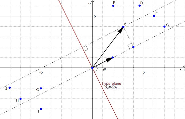
Let's calculate the distance between point A and the hyperplane. We begin this process by projecting point A onto the hyperplane.
Point A is a vector from the origin to A. So if we project it onto the normal vector w:
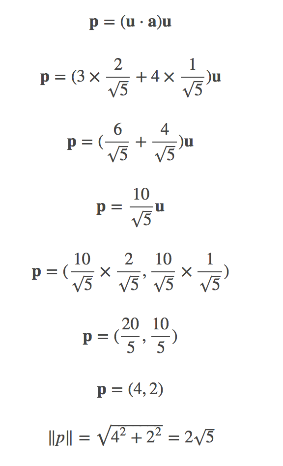
This will get us the projected vector! With the points (3,4) and (2,1) [this came from w = (2,1)], we can compute ||p||. Now, it'll take a few steps before we get there.
We begin by computing ||w||:
||w|| = √(22 + 12) = √5. If we divide the coordinates by the magnitude of ||w||, we can get the direction of w. This makes the vector u = (2/√5, 1/√5).
Now, p is the orthogonal prhoojection of a onto w, so:
1.3.2 Margin Computation
Now that we have ||p||, the distance between A and the hyperplane, the margin is defined by:
margin = 2||p|| = 4√5. This is the margin of the hyperplane!
Resources
If you want to learn more, stay tuned for further posts by me. Also feel free to visit my GitHub for more content on Data Science, Machine Learning, and more.
