Using harmonic modulation for N=1 experiments (Part 1/3)

Using harmonic modulation for N=1 experiments (Part 1/3)

This post got prompted by me trying to look for a good primer for Dave Feldman on the subject. Dave asked me to link to a good primer, but unfortunately, all of the best primers seem to be written from an electronics perspective, what isn't all that bad but might be a bit distracting if you want to apply the theory to your own diet and health-related N=1 experiment. In this post, I will try to discuss the subject of harmonic modulation in a way that is 100% black box based. That is, I'll try to explain it in such a way that it applies equally well to your body as black box as it does when applied to an analog electronic circuit.

I am breaking this blog up into three posts.

• An intro into black box analysis with harmonic signals.
• Partial reconstruction of transposition functions
• Use of these theories in health-oriented N=1 experiments, the engineering way.

These blog posts are written for people with at least some engineering knowledge who know how to program. It is not meant for hard math lovers. I will intentionally be cutting corners on the math part and simply demonstrate how to use simple code to get all the work done without necessarily understanding fully what is going on under the hood.

This is the first time that I'll write a blog post in Jupyter Notebook. Given that its a quite technical subject that benefits I think from example code and graphical representations, and given that Python is a far more common programming language for engineers doing things other than data engineering than some of the alternatives I have at my disposal, the use of Jupyter Notebook with Python 3 seems like a decent combo. Having said that, I'll just consider it a pilot post for making blog posts this way, if it doesn't work it doesn't work and I'll go back to keeping code and blogs seperate.

The best way to explain the concept is by creating a box that we understand. We will be applying a modulated signal to the box later to input X while monitoring output Y. While many studies in medical and nutritional science, from a design perspective, seem to assume a lineair relationship between two such variables, such a lineair relationship won't help us explain all of the important aspect of harmonic modulation based experiments. So let us start of by defining a non-lineair yet simple transpositional function between something of what our input is a component and a contributor to our output:

%matplotlib inline
import math
import numpy as np
import matplotlib.pyplot as plt

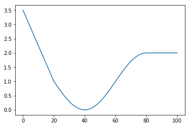
def transpose(x):
    if x < 20:
        return 3.5 - x/8
    if x > 80:
        return 2
    return 1 - math.sin((x-20)*math.pi/40)

x = numpy.linspace(0,100,num=100)
y = np.array([transpose(xi) for xi in x])
plt.plot(x, y)

[<matplotlib.lines.Line2D at 0x7ff7f1c860b8>]

Naturally, our transposition function won't be this obvious when we try to do actual controled measurements on it. We are talking relatively complex systems here. Lets look what happens if we add some system harmonics and randomness to our little box.

def complex_transpose(x,t):
    input_harmonic = 13 * math.sin(t/200) + 29 * math.cos(t)
    input_noice = np.random.normal(0, 17, size=1)[0]
    internal_x = x + input_harmonic + input_noice
    internal_y = transpose(internal_x)
    output_harmonic = math.cos(3*t+math.pi/5)
    output_noice = np.random.normal(0, 0.8, size=1)[0]
    rval = internal_y + output_harmonic + output_noice
    if rval < 0:
        return 0
    else:
        return rval

t = 0
def quick_transpose(x):
    global t
    rval = complex_transpose(x,t)
    t += 1
    return rval

def slow_transpose(x):
    global t
    rval = complex_transpose(x,t)
    t += 1000
    return rval
    
x = numpy.linspace(0,100,num=100)
y = np.array([quick_transpose(xi) for xi in x])
y2 = np.array([slow_transpose(xi) for xi in x])
plt.plot(x, y)
plt.plot(x, y2)

[<matplotlib.lines.Line2D at 0x7ff7f1c2f278>]

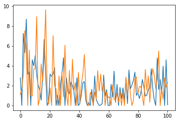
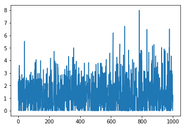
We try to reconstruct our transposition function, twice. Once quickly, once slow. But to no prevaill, our system is just to noicy to get anything usefull from at this point. Or is it? Let us start off by keeping our input stable and measuring the output for a little bit of time:

t = np.linspace(0,1000,num=1000)
y = np.array([complex_transpose(50,ti) for ti in t])
plt.plot(t, y)

[<matplotlib.lines.Line2D at 0x7ff7f0c5af98>]

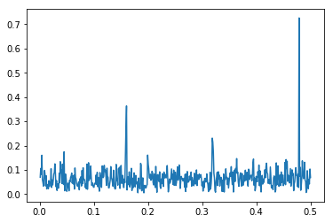
Looks pretty noicy, right, but then there is a hint of patterns. With our human minds, seeing spurious patterns is in our genes, so lets look what fourrier has to say.

from scipy.fftpack import fft

N = len(y)
T = 1
yf = fft(y)
absyf = 2.0/N * np.abs(yf[0:N//2])
xf = np.linspace(0.0, 1.0/(2.0*T), N//2)
plt.plot(xf[1:], absyf[1:])

[<matplotlib.lines.Line2D at 0x7ff7f0bc14a8>]

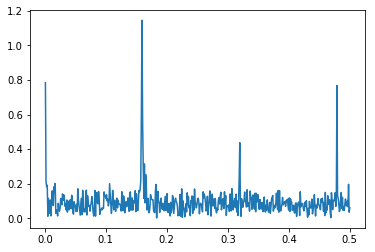
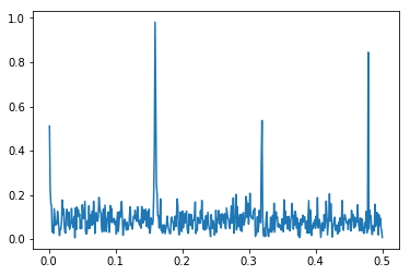
If we run the last two steps again and again, the noice will differ, but the system harmonics remain the same. So whate are we actually looking at? We are looking at the spectrum of the output signal given a stable input at a level of 50. If we have time, we might want to look at the same for a different an input level. As this is just a blog and all measurements are simulated, lets look at the same experiment for the levels of 25 and 75.

y = np.array([complex_transpose(25,ti) for ti in t])
yf = fft(y)
absyf = 2.0/N * np.abs(yf[0:N//2])
plt.plot(xf[1:], absyf[1:])

[<matplotlib.lines.Line2D at 0x7ff7f0b97fd0>]

y = np.array([complex_transpose(27,ti) for ti in t])
yf = fft(y)
absyf = 2.0/N * np.abs(yf[0:N//2])
plt.plot(xf[1:], absyf[1:])

[<matplotlib.lines.Line2D at 0x7ff7f0ff64e0>]

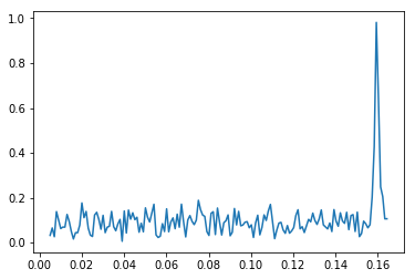
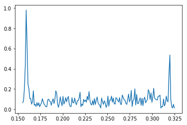
While the amplitudes differ significantly, notice we see the same three main peaks popping up every time. So what do we do next? Now that we have found the internal harmonics of our system, we go and find ourself a nice and quit spot on the spectrum. Let us see if we can zoom in a bit on a potential region.

plt.plot(xf[5:165], absyf[5:165])

[<matplotlib.lines.Line2D at 0x7ff7f03f5780>]

plt.plot(xf[155:325], absyf[155:325])

[<matplotlib.lines.Line2D at 0x7ff7f01b4c18>]

Now let us pick two silent places on the spectrum where we can introduce harmonic input signals to the system. It is important to not use frequencies that are multiples of eachother.
And if possible, frequencies that have the sample freqency as multiple should be avoides as well. Using fractions made of non repeprime numbers can be a simple strategy here.

We pick:

• 3/13 (0.231)
• 5/127 (0.0394)

Please note that because of the effects harmonic distortions due to possible non-linear transpositions, you will want to consider where A+B and A-B frequencies might end up with respect to the chosen and the already present frequencies. Avoid any situation where some sum of the frequencies involved and/or their negatives ends up too close to any of the other frequencies.

So if there is a system frequency of five, choosing two and seven as input harmonics would be unwise for the reason that two plus five is seven and harmonic distortion has properties that will have the three suposedly independent frequencied interact in ways that hinder our analysis.

def harmonic_transpose(x,t):
    h1 = 25 * math.sin(3 * t * 2 * math.pi/ 13)
    h2 = 25 * math.sin(5 * t * 2 * math.pi / 127)    
    return complex_transpose(x + h1 + h2 ,t)

y1 = np.array([complex_transpose(50,ti) for ti in t])
y2 = np.array([harmonic_transpose(50,ti) for ti in t])
yf1 = fft(y1)
yf2 = fft(y2)
absyf1 = 2.0/N * np.abs(yf1[0:N//2])
absyf2 = 2.0/N * np.abs(yf2[0:N//2])
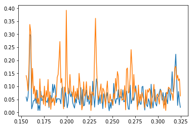
plt.plot(xf[155:325], absyf1[155:325])
plt.plot(xf[155:325], absyf2[155:325])

[<matplotlib.lines.Line2D at 0x7ff7f0fa7d30>]

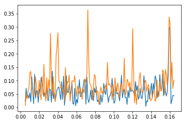
plt.plot(xf[5:165], absyf1[5:165])
plt.plot(xf[5:165], absyf2[5:165])

[<matplotlib.lines.Line2D at 0x7ff7ef8586a0>]

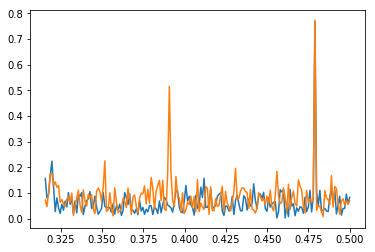
plt.plot(xf[315:], absyf1[315:])
plt.plot(xf[315:], absyf2[315:])

[<matplotlib.lines.Line2D at 0x7ff7ef4fa5c0>]

One thing sticks out. Apart from the three old freqencies and the two new ones, there are quite a few new ones as well.
These, most likely will be the result of harmonic distortions. Looking closely we could see that adding and subtracting the original frequencies will get us frequencies pretty close to the ones we are seeing. Basically seeing these sum and difference frequencies are a tell-tale sign of a non lineair transposition.

So what have we shown so far about our black box? We have shown that out output is responsive to our input, and we have shown it is so in a non lineair way.
This is important knowledge, as it helps us plan our next step.

In my upcomming blog in this series we will try to partially reconstruct out blackbox its transposition function.