Cryptocurrency Trading Bot Part 2 - TA-LIB Setup and Beginning Strategy
Where We Are Now?
If you have followed Step 1, then you now have a Binance client setup in Python. The next logical step is to develop a strategy to teach our bot how to trade. The strategy that we will develop today will sadly not make you a millionaire, but utilizing the principles learned in this tutorial in combination with indicator strategies and back testing methods which we will develop in future tutorials just might, so this is an important first step for our bot.
Indicators
The key to building any good trading strategy starts with good indicators. There are thousands of them out there, and luckily for us, we won't have to reinvent the wheel to access them because we have access to historical data in the form of the Binance API, and we will soon have TA-LIB which will give us access to these indicators in the form of a handy Python library.
Step 1 - Installing TA-Lib and MatplotLib
TA-Lib (short for Technical Analysis Library) can be installed by simply running the command:
pip install TA-Lib
This instillation is notorious for running into issues, but luckily many people have failed with this very same installation so if you have problems, check the troubleshooting section on the Github page, or do a quick google search of any error produced by the installation and you should find a solution.
We will be using MatPlotLib to create plots and other analytics moving forward. MatPlotLib can be installed with:
pip install matplotlib
Numpy is a helpful library for doing a number of necessary array and matrix operations among other things, and can be installed with:
pip install numpy
The final two libraries we will need are pandas and pandas_datareader. These libraries will simplify the task of converting data pulled from the Binance API into a format which TA-Lib can compute from. We will not use these libraries today for our simple example, but they will come in handy later. These libraries can be installed with:
pip install pandas
pip install pandas_datareader
Step 2 – Generate First Indicator
Now we will use the data pulled from the Binance API in combination with TA-Lib, Numpy, and MatPlotLib to generate a MACD plot for the BTC/USDT trading pair. MACD stands for moving average convergence divergence. It is a trend-following momentum indicator that shows the relationship between two moving averages of prices. We will plot these two moving average lines with the following modified python script which we started in the previous part.
from binance.client import Client
import talib as ta
import matplotlib.pyplot as plt
import numpy as np
from datetime import datetime

class Trader:
    def __init__(self, file):
        self.connect(file)

    """ Creates Binance client """
    def connect(self,file):
        lines = [line.rstrip('\n') for line in open(file)]
        key = lines[0]
        secret = lines[1]
        self.client = Client(key, secret)

    """ Gets all account balances """
    def getBalances(self):
        prices = self.client.get_withdraw_history()
        return prices

filename = 'credentials.txt'
trader = Trader(filename)

trading_pair = 'BTCUSDT'
interval = '1d'
klines = trader.client.get_klines(symbol=trading_pair,interval=interval)
open_time = [int(entry[0]) for entry in klines]
close = [float(entry[4]) for entry in klines]
close_array = np.asarray(close)
new_time = [datetime.fromtimestamp(time/1000) for time in open_time]

macd, macdsignal, macdhist = ta.MACD(close_array, fastperiod=12, slowperiod=26, signalperiod=9)


plt.style.use('dark_background')
plt.plot(new_time, macd, label='MACD')
plt.plot(new_time, macdsignal, label='MACD Signal')
plt.plot(new_time, macdhist, label='MACD Histogram')
plt.title("MACD Plot for BTC/USDT")
plt.xlabel("Open Time")
plt.ylabel("Value")
plt.legend()
plt.show()
In future tutorials we will move code for data generation, indicator computing, and plotting into separate classes and functions to make it easier to build complex trading strategies, but for now this code will be fine at the module level.
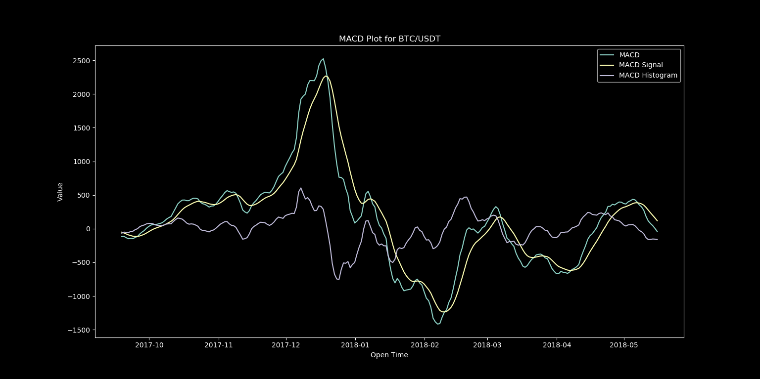
If all of your libraries have been installed successfully, you should see an output that looks like this:

Figure 1: MACD output from above code
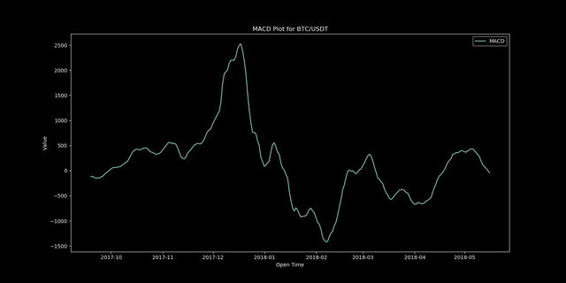
By pulling up the MACD computed by TradingView, we can compare this to our isolated MACD line:

Figure 2: Isolated MACD Line from above code

Figure 3: MACD Output From TradingView
An exact match, this means that we are now successfully able to compute the MACD indicator and can use it to build our very first trading strategy!
Step 3 – Crafting a Strategy
The strategy that we will be creating will be a simple MACD crosover trading strategy. The idea is fairly simple and looks at the relationship between the MACD line and the MACD signal line (also called the trigger line). There are two types of crossovers:
- Bullish MACD Crossover – We have a bullish MACD crossover when the MACD line crosses the slower signal line in the bullish direction. This action generates a bullish signal on the chart, which implies that the price might start an increase.
- Bearish MACD Crossover – The bearish MACD crossover is opposite to the bullish MACD crossover. When the MACD line crosses the signal line in the bearish direction, we have a bearish crossover. This hints that the price action might be entering a bearish move.
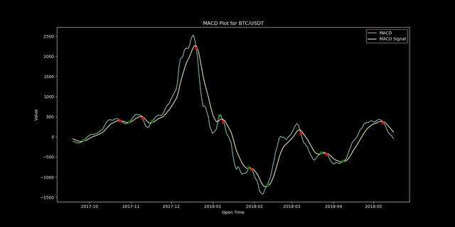
To start, we will add red and green indicators to our plot to show these crossover point. We can do this by replacing the code beneath this line:
macd, macdsignal, macdhist = ta.MACD(close_array, fastperiod=12, slowperiod=26, signalperiod=9)
with this:
crosses = []
macdabove = False
for i in range(len(macd)):
    if np.isnan(macd[i]) or np.isnan(macdsignal[i]):
        pass
    else:
        if macd[i] > macdsignal[i]:
            if macdabove == False:
                macdabove = True
                cross = [new_time[i],macd[i],'go']
                crosses.append(cross)
        else:
            if macdabove == True:
                macdabove = False
                cross = [new_time[i],macd[i],'ro']
                crosses.append(cross)


plt.style.use('dark_background')
plt.plot(new_time, macd, label='MACD')
plt.plot(new_time, macdsignal, label='MACD Signal')
for cross in crosses:
    plt.plot(cross[0],cross[1],cross[2])
#plt.plot(new_time, macdhist, label='MACD Histogram')
plt.title("MACD Plot for BTC/USDT")
plt.xlabel("Open Time")
plt.ylabel("Value")
plt.legend()
plt.show()
After running this code, we get the following:

Figure 4: MACD crossover strategy
This code for locating crossover points will certainly be improved in future posts, but this is a good start, and locating these points will make it very easy to backtest this trading strategy.
Looking Ahead
In the next installment in this series, we will be cleaning up the code to generate our indicators into more versatile functions and classes, adding support for more indicators, and begin creating our backtesting tools to analyze the performance of various strategies.
Looking even further ahead, I'll be covering:
- Making our bot run in realtime
- Expanding backtesting and analytics to read and write data to a MySQL database
- Many more trading strategies
- More efficient methods for scanning multiple trading pairs
- Using TensorFlow to utilize machine learning for tuning weight of indicators in deciding on potential trades
- And much more
Any requests for future topics to cover or general feedback are greatly appreciated.
Thanks for reading,
Andrew
Do you plan on simulating stop losses / take profits on your strategies ?
Right now I can see 9 signals out of 16 are good (for the strategy you presented), so you'll have to implement stop-losses. Or maybe hedging with leverages, I don't know which can be the most efficient.
There's a lot of sudden movements in these markets that can easily trigger a stop loss if too tight.
Will you try some more short-term strategies too ?
Anyway, looking forward to hear more about your tests !
Yes, adding stop losses will definitely be a high priority, and will be even more helpful when trading on shorter intervals. I typically like to trade on the 15m and 1h intervals so a lot of the strategies I'll be posting moving forward will be centered around those.